Discretization

The simulation domain is discretized into four zones along the borehole depth. Upper and lower layers are axial only, while the ground and borehole domains are discretized both axially and radially.

Overview

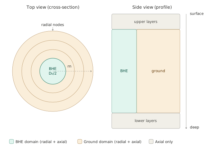
Upper layers

Axial nodes only — no radial discretization. Each node represents a single temperature for the ground above the active borehole section. These layers account for the thermal mass between the surface and the borehole top. The upper node is the surface one.

Ground domain

m_mesh axial layers, each containing n_mesh radial nodes. The domain extends radially from the borehole wall to the far-field boundary rn. Stored row-major: all n_mesh radial nodes of axial layer 0, then layer 1, and so on.

Borehole domain

m_mesh axial nodes, each described by a local system of n_equations, known basing on the chosen configuration. The number of equations and their positions within each node block depend on the BHE type:

BHE type	n_equations	shell	core	shell middle	fluid down	fluid up
SingleUtube	6	0	1	n.d.	4	5
DoubleUtube	10	0	1	n.d.	8	9
Coaxial	5	0	n.d.	n.d.	3	4
Helical	7	0	1	2	5	6

The offsets n_equations - 2 and n_equations - 1 always point to fluid down and fluid up respectively. If the BHE is Coaxial or Helical, check which is the inlet pipe to adjust indexes.

Lower layers

Axial nodes only — no radial discretization. Symmetric to the upper layers, representing the deep ground below the active borehole section.

Initial and boundary conditions

The initial temperature field and the far-field boundary condition are both derived from the Kusuda-Achenbach analytical model [Kusuda1965]. At the start of the simulation, every node in the domain is initialised with the temperature predicted by this model at the corresponding depth and time. The same profile is used as the far-field radial boundary condition at rn for single-borehole mode throughout the simulation, so the outer boundary always follows the undisturbed seasonal ground temperature cycle rather than a fixed value.

In multi-borehole mode (with series connection or irregular spacing) the far-field boundary is updated at each timestep by the FLS thermal interference model (see FLS Calculation Methods), which adds thevinter-borehole temperature perturbation on top of the Kusuda-Achenbach baseline. If the boreholes are regularly spaced and connected in parallel, the adiabatic condition will be used at mid-distance between adjacent boreholes.

[Kusuda1965]

Kusuda, T., Achenbach, P.R. (1965). Earth temperature and thermal diffusivity at selected stations in the United States. ASHRAE Transactions, 71(1).